Tutorial 5c – 2D FE-plate with spatially uncertain Young's modulus
In this tutorial we use Fesslix to model a 2D FE-plate that has a spatially uncertain Young's modulus.
The random field is discretized and a reliability analysis is performed.
Table of Contents
1 Mechanical model
This tutorial is based on the mechanical model employed in Tutorial 4c.
Compared to Tutorial 4c, the Young's modulus is no loger constant:
It is modeled as a log-Normal random field that has mean  and standard deviation
  .
.
We model the log-Normal random field by means of an underlying Gaussian random field. The auto-correlation coefficient function is isotropic and of exponential squared type; the correlation length is 0.5m.
Additionally, the loading q is modeled as a random field with a marginal distribution that is Gumbel. The mean and standard deviation of q is 50kN/m and 20kN/m, respectively. The random field is modeled by means of an underlying Gaussian random field. The auto-correlation coefficient function is isotropic and of exponential squared type; the correlation length is 1.5m.
Note: A similar problem is discussed in [1].
and standard deviation .
We model the log-Normal random field by means of an underlying Gaussian random field. The auto-correlation coefficient function is isotropic and of exponential squared type; the correlation length is 0.5m.
Additionally, the loading q is modeled as a random field with a marginal distribution that is Gumbel. The mean and standard deviation of q is 50kN/m and 20kN/m, respectively. The random field is modeled by means of an underlying Gaussian random field. The auto-correlation coefficient function is isotropic and of exponential squared type; the correlation length is 1.5m.
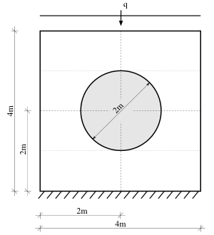
Figure 1: The plate problem from Tutorial 4c is investigated, assuming that the Young's modulus of the plate is spatially uncertain.
Note: A similar problem is discussed in [1].
2 Step by Step Instruction
2.1 Define the mesh
It is suggested to make the following changes compared to Tutorial 4c:
Set the variables ref_x and ref_y to 1.0; i.e.:
Fesslix parameter file
# Control the mesh size
  const ref_x = 1.0;    # mesh-refinement in horizontal direction
  const ref_y = 1.0;    # mesh-refinement in vertical direction
2.2 Random field discretization
Fesslix parameter file
#! ===============================
#! Random field discretization (FE-KL)
#! ===============================

#! -------------------------------
#! Young's modulus
#! -------------------------------

const M = 100;   # number of terms in expansion
const a = 0.5;   # correlation length
const pO = 8;   # polynomial order of the FE shape functions

# type of discretization: finite element KL expansion
  rf_new 1 kl_fem_gauss mu 0.0 sd 1.0 rhocor autocorr_exp2(deltap,a);
    # where deltap is the distance between two RF-points
# Assign a geometry to the field:
  for (i=1;i<4.5;i+1) {
    rf_elset 1 face i porderLx=PO porderLy=PO tensorspace=true {dolog=false;};
  };
# Obtain the random field discretization
  rf_solve 1 dim=M;
# transform to log-Normal space
  var rf_E = rnd_y2x(rf(1), logn, mu=3e7, sd=0.6e7);

#! -------------------------------
#! Loading
#! -------------------------------
const a2 = 1.5;   # correlation length

# type of discretization: finite element KL expansion
  rf_new 2 kl_fem_gauss mu 0.0 sd 1.0 rhocor autocorr_exp2(deltap,a2);
    # where deltap is the distance between two RF-points
# Assign a geometry to the field:
  rf_elset 2 edge 5 porder=PO { dolog=false; };
  rf_elset 2 edge 6 porder=PO { dolog=false; };
# Obtain the random field discretization
  rf_solve 2 dim=5;
# transform to Gumbel space
  var rf_q = -rnd_y2x(rf(2), gumbel, mu=70, sd=35);
2.3 Define finite elements of mechanical model
Fesslix parameter file
#! ===============================
#! Define the finite elements
#! ===============================

# Material definition
  isomat 0 E rf_E nu 0.15 { degreeE=pO; };

# Plane stress FE-elements
  elplanestr 1 1 {          # element 1 in face 1
      material    = 0;        # the material-number to assign to the element
      t           = 0.1;      # plate thickness [m]
      planestress = true;     # true: plane stress; false: plaine strain
    };
elplanestr 2 2 { t=0.1; };
elplanestr 3 3 { t=0.1; };
elplanestr 4 4 { t=0.1; };
2.4 Define the loads
Fesslix parameter file
#! ===============================
#! Define the loads
#! ===============================
# Apply uniformly distributed load of 5kN/m on top of plate:
  eload 5 local wy pos=[-1,1] load=rf_q;
  eload 6 local wy pos=[-1,1] load=rf_q;
2.5 Solve the system
Fesslix parameter file
#! ===============================
#! Solve the system
#! ===============================

fem assdof;          # assemble degrees of freedom

sub fesolve() {
  fem assstf { dolog=false; };    # assemble stiffness matrix
  fem assforces { dolog=false; }; # assemble forces
  fem solve {                     # solve the system
    printsol=false;      # setting this to true will output the entire solution vector
    pcn=4;               # employ a direct solver
    dolog =false;
  };
};

# Solve for a random realization
  rnd_smp "rf_1";
  rnd_smp "rf_2";
  fesolve();
  # output the displacement at the upper left and right corner of the plate
    funplot nodeu([6,wy]), nodeu([8,wy]), nodeu([6,wx]), nodeu([8,wx]);
2.6 Reliability analysis
As last step we perform a reliability analysis (see Tutorial 1).
Failure occurs if the displacement in the middle of the upper plate edge exceeds 2mm.
Subset Simulation is employed to approximate the probability of failure.
Subset Simulation is employed to approximate the probability of failure.
Fesslix parameter file
#! ===============================
#! Reliability analysis
#! ===============================

#! -------------------------------
#! Limit-state functon
#! -------------------------------
const t = 1e-3;   # maximum allowable displacement at node 7

var lsf = t+objexec(nodeu([7,wy]),{
    fesolve();
  });

 # evaluate limit-state function for current realization
   funplot lsf, nodeu([7,wy]);


#! -------------------------------
#! Subset simulation
#! -------------------------------
loadlib "RND";

const Nsmp = 1e3;  # number of samples used per level in Subset Simulation
const pthr = 10%;  # probability of the intermediate Subset levels

sus (
  Nsmp*pthr;               # The number of chains used at each level in Subset Simulation.
  1/pthr;                  # The length of each chain.
  lsf                      # The limit-state function.
) {
  rbrvsets = "rf_1,rf_2";  # The sets of random variables to use.
};
# Note: it will take some time to finish the computation ...
3 The complete input files of this tutorial

4 References
- [1] Betz, W. & Papaioannou, I. & Straub, D. (2014). Numerical methods for the discretization of random fields by means of the Karhunen-Loeve expansion. Comput. Methods Appl. Mech. Engrg., 109-129. (download manuscript)