Tutorial 5b – Inhomogeneous one-dimensional log-Normal random field
In this tutorial we use Fesslix to discretize a inhomogeneous one-dimensional log-Normal random field.
For this tutorial you must have a 64-bit version of Python 2.7 installed on your system.
You can download the latest 2.7 release from here: https://www.python.org/downloads/windows/.
Table of Contents
1 Random field properties
The goal is to represent a log-Normal random field that has mean 10 and standard deviation function
 .
We assume that the random field can be transformed to an underlying Gaussian random field; i.e.,
by taking the natural logarithm of the log-Normal random field.
The auto-correlation coefficient function of the underlying Gaussian random field is:
.
We assume that the random field can be transformed to an underlying Gaussian random field; i.e.,
by taking the natural logarithm of the log-Normal random field.
The auto-correlation coefficient function of the underlying Gaussian random field is:
 .
The domain of interest has a length of 3m.
.
The domain of interest has a length of 3m.
.
We assume that the random field can be transformed to an underlying Gaussian random field; i.e.,
by taking the natural logarithm of the log-Normal random field.
The auto-correlation coefficient function of the underlying Gaussian random field is:
.
The domain of interest has a length of 3m.
2 Step by Step Instruction
Note: This tutorial uses the Python plotting library matplotlib. If you do not have Python and matplotlib installed on your system, you have to comment-out the corresponding lines in the Fesslix parameter file.
2.1 Random field discretization
Fesslix parameter file
#! ===============================
#! Load the FE module
#! ===============================

loadlib "fem";

#! ===============================
#! Initial definitions
#! ===============================

const l  = 3;              # [m] length of random field domain
const mu = 10;             # mean value of random field
var sd = 4*(gx-1.5)^2+1;   # std. dev. function of random field

# auto-correlation coefficient function of underlying Gaussian field
var corr = exp(-1*(deltap/(min((min(gx,gx2)/1.5)^4,2)+0.1))^2);

const M  = 10;     # number of terms in the random field expansion

# mean of underlying Gaussian field
  fun lambda(2) = ln($1)-ln(($2/$1)^2+1)/2;
# std. dev. of underlying Gaussian field
  fun chi(2)    = sqrt(ln(($2/$1)^2+1));


#! ===============================
#! Define the mesh
#! ===============================
# The mesh becomes finer from right to left.

const Nel = 20;
const x = 1;
fun xf(2) = $1*(1-1/$2)^(($2/Nel)^8*1+1);
for (i=Nel;i>0.5;i-1) {
  node i [l*x];
  funplot i, l*x;
  const x = xf(x,i);
};
node 0 [0];
for (i=1;i<Nel+0.5;i+1) {
  edge i i-1 i;
};


#! ===============================
#! Random field discretization (FE-KL)
#! ===============================

const pO = 10;   # polynomial order of the FE shape functions
const MO = 0.1;  # 1/MO is number of sub-intervals in outer integration loop

# type of discretization: finite element KL expansion
  rf_new 1 kl_fem_gauss mu lambda(mu,sd) sd chi(mu,sd) rhocor CORR;
# Assign a geometry to the field:
  for (i=1;i<Nel+0.5;i+1) {
    rf_elset 1 edge i porder=PO MAXSIZEO=MO {dolog=false;};
  };
# Obtain the random field discretization
  rf_solve 1 dim=M calcerr=false;

funplot #rf_err(1,1),
  rf_err(1,101),      # Var-based measure - used instead of '1' as std.dev. varies
  rf_err(1,2),        # Cov-based measure
  rf_err(1,3);        # error measure 3
2.2 Output Eigenvalues
Fesslix parameter file
#! ===============================
#! Output eigenvalues
#! ===============================

const NEV = M;
sfor (i;NEV) {
  funplot i, rf_eigenvalue(1,i);
};
2.3 Plot the eigenmodes of the random fields
Fesslix parameter file
#! ===============================
#! Plot the eigenmodes of the random fields
#! ===============================

#! -------------------------------
#! output the eigenmodes to files
#! -------------------------------

const ppd = 500;                # number of points to use for plotting
mtxconst_new ppd1(3,1,ppd/Nel); # ... for 2nd random field

filestream fs ("output_rf2.dat");
rf_plot 1 { ppdim = ppd1; stream=fs; };


#! -------------------------------
#! invoke the tool matplotlib
#! -------------------------------
# You can comment this section out if you do not have
# 'Python' or 'matplotlib' installed on your system.

# load the python-module
  loadlib "Python";
# add current path to Python search path
  python_path $pwd();
# load the module 'tutorial_1d_lsf'
  python_module tutorial_5b_plot;
# link the Python function to Fesslix
  python_fun plot_fun = tutorial_5b_plot.PlotModes;
# start the plotting
  calc plot_fun();
Again, as in the previous tutorial (Tutorial 5a), Python with the plotting library matplotlib is used.
The corresponding Python code is given at the end of this tutorial.
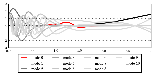
Figure 1: Plot of the eigenmodes of the random field.
2.4 Plot covariance around 1.5m
Fesslix parameter file
#! ===============================
#! Plot covariance around 1.5
#! ===============================
# of the underlying Gaussian random field!!!

#! -------------------------------
#! output the covariance structure
#! -------------------------------

filestream fs ("output_rf_cov.dat");
rf_plotcov 1 [1.5] {stream=fs;};

#! -------------------------------
#! invoke the tool matplotlib
#! -------------------------------
# You can comment this section out if you do not have
# 'Python' or 'matplotlib' installed on your system.

# link the Python function to Fesslix
  python_fun plot_cov = tutorial_5b_plot.PlotCov;

calc plot_cov();

Figure 2: Plot of the covariance around x=1.5m.
2.5 Plot realizations
Fesslix parameter file
#! ===============================
#! Plot realizations
#! ===============================

#! -------------------------------
#! generate realizations
#! -------------------------------
const Nrep = 10;
const Npel = 20;
mtxconst_new resv(Nel*(Npel+1),Nrep+1,0);
sfor (j;Nrep) {
  const c = 0;
  rnd_smp "rf_1";
  for (i=1;i<Nel+0.5;i+1) {
    for (lx=-1;lx<=1;lx+2/Npel) {
      const res = geocalc(edge,i,exp(rf(1)),lx);
      mtxcoeff resv(c,0) = gx;
      mtxcoeff resv(c,j) = res;
      const c += 1;
    };
  };
};

#! -------------------------------
#! output the realizations
#! -------------------------------
filestream fs("output_reali.dat");
sfor (j;Nel*(Npel+1)) {
  mtxconst_sub vsub = resv(row:j);
  funplot {vsub} { stream=fs; };
};

#! -------------------------------
#! invoke the tool matplotlib
#! -------------------------------
# You can comment this section out if you do not have
# 'Python' or 'matplotlib' installed on your system.

# link the Python function to Fesslix
  python_fun plot_reali = tutorial_5b_plot.PlotReali;

calc plot_reali();
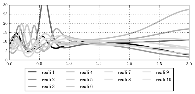
Figure 3: Plot of random field realizations.
2.6 Python code
The Python code used to generate the plots is:
Python code "tutorial_5b_plot.py"
# -*- coding: utf-8 -*-
import flx;
import matplotlib.pyplot as plt
import matplotlib as mpl
import numpy as np
import matplotlib.patches as mpatches

from matplotlib.backends.backend_pgf import FigureCanvasPgf
mpl.backend_bases.register_backend('pdf', FigureCanvasPgf)

pgf_with_pdflatex = {
    "pgf.texsystem": "pdflatex",
    "pgf.preamble": [
         r"\usepackage[utf8x]{inputenc}",
         r"\usepackage[T1]{fontenc}",
#         r"\usepackage{cmbright}",
         ]
}
mpl.rcParams.update(pgf_with_pdflatex)

def PlotModes():
  # =====================================
  # Read data from files
  # =====================================
  dfile = r'output_rf2.dat'
  m = {}
  x, er, m[1], m[2], m[3], m[4], m[5], m[6], m[7], m[8], m[9], m[10] = np.genfromtxt(
     dfile, unpack=True, usecols=(0,3,4,5,6,7,8,9,10,11,12,13))
  # =====================================
  # Do the plotting
  # =====================================
  plt.rc('text', usetex=True)
  plt.rc('font', family='roman', size=10)
  plt.figure(1, figsize=(6.3,2.5))
  plt.grid(True)
  plt.plot(x, er, linewidth=3, color='red', label=r'mode 0')
  for i in range (1,11):
    plt.plot(x, m[i], linewidth=3, color="{:.9f}".format(pow(1.-(1./i),1.3)),
	     label=r'mode '+"{:.0f}".format(i))
  plt.xlabel(r'$x$')
  art = []
  legend = plt.legend(loc=9, bbox_to_anchor=(0.5, -0.1),ncol=4)
  art.append(legend)
  for label in legend.get_texts():
    label.set_fontsize('medium')
  for label in legend.get_lines():
    label.set_linewidth(2)  # the legend line width
  plt.tight_layout()
  plt.savefig('tutorial_5b_plot_modes.pdf', format='pdf', additional_artists=art,
	      bbox_inches="tight")
  plt.savefig('tutorial_5b_plot_modes.png', format='png', additional_artists=art,
	      bbox_inches="tight")
  plt.show()
  return 0;

def PlotReali():
  # =====================================
  # Read data from files
  # =====================================
  dfile = r'output_reali.dat'
  m = {}
  x, m[1], m[2], m[3], m[4], m[5], m[6], m[7], m[8], m[9], m[10] = np.genfromtxt(
     dfile, unpack=True, usecols=(0,1,2,3,4,5,6,7,8,9,10))
  # =====================================
  # Do the plotting
  # =====================================
  plt.rc('text', usetex=True)
  plt.rc('font', family='roman', size=10)
  plt.figure(1, figsize=(6.3,2.5))
  plt.grid(True)
  for i in range (1,11):
    plt.plot(x, m[i], linewidth=3, color="{:.9f}".format(pow(1.-(1./i),1.3)),
	     label=r'reali '+"{:.0f}".format(i))
  plt.xlabel(r'$x$')
  plt.ylim([0,30])
  art = []
  legend = plt.legend(loc=9, bbox_to_anchor=(0.5, -0.1),ncol=4)
  art.append(legend)
  for label in legend.get_texts():
    label.set_fontsize('medium')
  for label in legend.get_lines():
    label.set_linewidth(2)  # the legend line width
  plt.tight_layout()
  plt.savefig('tutorial_5b_plot_reali.pdf', format='pdf', additional_artists=art,
	      bbox_inches="tight")
  plt.savefig('tutorial_5b_plot_reali.png', format='png', additional_artists=art,
	      bbox_inches="tight")
  plt.show()
  return 0;

def PlotCov():
  # =====================================
  # Read data from files
  # =====================================
  dfile = r'output_rf_cov.dat'
  m = {}
  x, m[1], m[2], m[3] = np.genfromtxt(dfile, unpack=True, usecols=(0,3,4,5))
  # =====================================
  # Do the plotting
  # =====================================
  plt.rc('text', usetex=True)
  plt.rc('font', family='roman', size=10)
  plt.figure(1, figsize=(6.3,2.5))
  plt.grid(True)
  plt.plot(x, m[1], linewidth=3, color="red", label=r'cov approx.')
  plt.plot(x, m[2], linewidth=3, color="black", label=r'cov analytical')
  plt.plot(x, m[3], linewidth=3, color="orange", label=r'difference')
  plt.xlabel(r'$x$')
  art = []
  legend = plt.legend(loc=9, bbox_to_anchor=(0.5, -0.1),ncol=4)
  art.append(legend)
  for label in legend.get_texts():
    label.set_fontsize('medium')
  for label in legend.get_lines():
    label.set_linewidth(2)  # the legend line width
  plt.tight_layout()
  plt.savefig('tutorial_5b_plot_cov.pdf', format='pdf', additional_artists=art,
	      bbox_inches="tight")
  plt.savefig('tutorial_5b_plot_cov.png', format='png', additional_artists=art,
	      bbox_inches="tight")
  plt.show()
  return 0;
3 The complete input files of this tutorial
